논문 개요
딥마인드에서 오디오 시그널에 대한 모델로 제시한 network 입니다. 해당 논문이 가지는 가장 큰 장점은 오디오의 waveform 자체 데이터를 활용해서 모델링을 수행한 점입니다. 또한 이를 통해 생성한 TTS는 기존의 결과보다 많이 나은 성능을 보여주고 있습니다. 최근에는 Google Home에 해당 네트워크가 탑제되었으며 wav 파일 관련해서 reference network로 많이 활용되고 있습니다. Paper Deepmind blog
Network Architecture 설명
네트워크를 이해하기 위해서는 해당 내용에 대한 개념을 먼저 이해해야 합니다.
- stack of dilated casual convolution
- Residual and skip connection
- softmax distribution
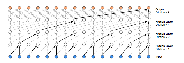
stack of dilated casual convolution
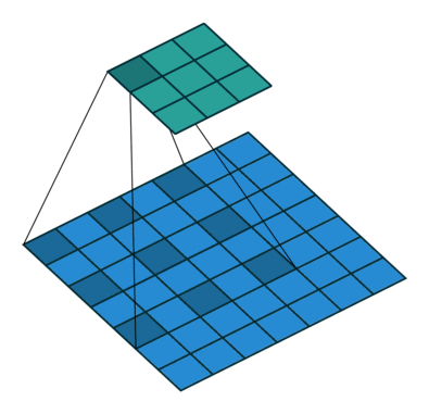
우선 WAV 데이터 형태는 1차원의 데이터 형태이기 때문에 CNN 적용 시 Conv1D 를 기본적으로 활용하고 있습니다. 해당 네트워크 구조를 이해하기 위해서는 우선적으로 dilation 개념에 대한 이해가 먼저 필요 합니다.
dilation의 의미는 CNN 수행 시 커널을 구성함에 있어서 커널의 Pixel 사이에 얼마나 빈 공간을 줄 것인가 하는 점입니다. 기본적으로 사용하는 커널은 dilation=1 이며 dilation 값이 추가 될 수록 커널 사이에 빈 공간이 추가 된다고 보시면 됩니다.
WaveNet에서 사용하는 stacked of dilated casual convolution의 경우 1D Conv를 누적으로 쌓는 형태를 기본으로 한 후 누적 시 마다 dilation의 값을 2의 배수 만큼 증가시키는 형태압니다. 이 때 사용하는 parameter가 depth 값이며 만약 depth =10 이면 1, 2, 4, 8, 16 ,…, 512 순서로 stack 작업을 수행합니다.
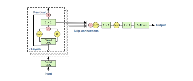
Residual and Skip connections
Input Data(x)가 네트워크로 들어오면 다음의 Process 과정을 거칩니다.
- tanh(x), sigmoid(x), skip_connection(x) 의 3가지 network path을 설정
- 3가지 path에 대해 Dilated Conv를 적용
- tanh와 sigmoid의 경우에는 Gate Activation Unit 방법을 적용
- 3의 결과에 1X1 Conv 적용
- 4의 결과와 Input Data(x)와 resudial 적용
- 5의 결과와 skip_connection(x)와 sum 적용
- 6의 결과에 대해 Relu - 1X1 Conv -Relu - 1X1 Conv - Softmax 를 적용하여 최종 Output을 산출
Softmax Disribution
WaveNet 적용 시 output class는 Audio의 timestep 별 integer 값 입니다. 하지만 이 값이 상당히 많은 range 값을 가지고 있습니다.(16bit의 경우에 65,534(2의 16제곱) 값을 가짐) 따라서 Output class 의 범위를 좁히는 과정이 필요한데 이 때 사용하는 방법이 $\mu$ -law companding transformation 입니다. 해당 방법을 적용하면 우리가 설정한 $\mu$ 값으로 class 범위를 줄일 수 있습니다.
Python을 이용한 구현
WaveNet을 구현하기 위해 다음의 Module을 lading 합니다.
%matplotlib inline
import numpy as np
from matplotlib import pyplot as plt
import mxnet as mx
from mxnet import gluon, autograd, nd
from mxnet.gluon import nn,utils
import mxnet.ndarray as F
from IPython.display import Audio
from scipy.io import wavfile
from tqdm import tqdm
import sys
WaveNet 구현을 위한 필요 Class를 정의 합니다. 우선적으로 integer 값을 one-hot 으로 변환하기 위한 class를 정의 합니다.
class One_Hot(nn.Block):
    def __init__(self, depth):
        super(One_Hot,self).__init__()
        self.depth = depth
    def forward(self, X_in):
        with X_in.context:
            X_in = X_in
            self.ones = nd.one_hot(nd.arange(self.depth),self.depth)
            return self.ones[X_in,:]
    def __repr__(self):
        return self.__class__.__name__ + "({})".format(self.depth)
다음으로 WaveNet Class를 정의 합니다.
class WaveNet(nn.Block):
    def __init__(self, mu=256,n_residue=32, n_skip= 512, dilation_depth=10, n_repeat=5):
        # mu: audio quantization size
        # n_residue: residue channels
        # n_skip: skip channels
        # dilation_depth & n_repeat: dilation layer setup
        super(WaveNet, self).__init__()
        self.dilation_depth = dilation_depth
        self.dilations = [2**i for i in range(dilation_depth)] * n_repeat
        with self.name_scope():
            self.one_hot = One_Hot(mu)
            self.from_input = nn.Conv1D(in_channels=mu, channels=n_residue, kernel_size=1)
            self.conv_sigmoid = nn.Sequential()
            self.conv_tanh = nn.Sequential()
            self.skip_scale = nn.Sequential()
            self.residue_scale = nn.Sequential()
            for d in self.dilations:
                self.conv_sigmoid.add(nn.Conv1D(in_channels=n_residue, channels=n_residue, kernel_size=2, dilation=d))
                self.conv_tanh.add(nn.Conv1D(in_channels=n_residue, channels=n_residue, kernel_size=2, dilation=d))
                self.skip_scale.add(nn.Conv1D(in_channels=n_residue, channels=n_skip, kernel_size=1, dilation=d))
                self.residue_scale.add(nn.Conv1D(in_channels=n_residue, channels=n_residue, kernel_size=1, dilation=d))
            self.conv_post_1 = nn.Conv1D(in_channels=n_skip, channels=n_skip, kernel_size=1)
            self.conv_post_2 = nn.Conv1D(in_channels=n_skip, channels=mu, kernel_size=1)

    def forward(self,x):
        with x.context:
            output = self.preprocess(x)
            skip_connections = [] # save for generation purposes
            for s, t, skip_scale, residue_scale in zip(self.conv_sigmoid, self.conv_tanh, self.skip_scale, self.residue_scale):
                output, skip = self.residue_forward(output, s, t, skip_scale, residue_scale)
                skip_connections.append(skip)
            # sum up skip connections
            output = sum([s[:,:,-output.shape[2]:] for s in skip_connections])
            output = self.postprocess(output)
        return output

    def preprocess(self, x):
        output = F.transpose(self.one_hot(x).expand_dims(0),axes=(0,2,1))
        output = self.from_input(output)
        return output

    def postprocess(self, x):
        output = F.relu(x)
        output = self.conv_post_1(output)
        output = F.relu(output)
        output = self.conv_post_2(output)
        output = nd.reshape(output,(output.shape[1],output.shape[2]))
        output = F.transpose(output,axes=(1,0))
        return output

    def residue_forward(self, x, conv_sigmoid, conv_tanh, skip_scale, residue_scale):
        output = x
        output_sigmoid, output_tanh = conv_sigmoid(output), conv_tanh(output)
        output = F.sigmoid(output_sigmoid) * F.tanh(output_tanh)
        skip = skip_scale(output)
        output = residue_scale(output)
        output = output + x[:,:,-output.shape[2]:]
        return output, skip
코드 구성은 앞에서 설명한 Process로 진행합니다. stack of dilated casual convolution을 수행한 후에 residual_forward를 거친 후 최종적으로 Softmax를 거쳐서 우리가 원하는 class별 확률 값을 산출합니다.
다음으로 Softmax Distribution 적용을 위한 Encoder/Decoder 함수를 정의합니다. 함수 내용은 앞에서 설명드린 수식을 코드로 표현한 결과 입니다.
def encode_mu_law(x, mu=256):
    mu = mu-1
    fx = np.sign(x)*np.log(1+mu*np.abs(x))/np.log(1+mu)
    return np.floor((fx+1)/2*mu+0.5).astype(np.long)

def decode_mu_law(y, mu=256):
    mu = mu-1
    fx = (y-0.5)/mu*2-1
    x = np.sign(fx)/mu*((1+mu)**np.abs(fx)-1)
    return x
다음으로 네트워크 학습을 위해 네트워크를 정의하고, parameter 및 Optimizer를 설정 합니다. Gluon에서 GPU를 사용하기 위해서는 별도의 context를 지정해주어야 하기 때문에 그 부분을 포함해서 코드를 작성합니다.
ctx = mx.gpu(1)
net = WaveNet(mu=128,n_residue=24,n_skip=128,dilation_depth=10,n_repeat=2)
net.collect_params().initialize(ctx=ctx)
#set optimizer
trainer = gluon.Trainer(net.collect_params(),optimizer='adam',optimizer_params={'learning_rate':0.01 })
g = data_generation(data,fs,mu=128, seq_size=20000,ctx=ctx)
batch_size = 64
loss_fn = gluon.loss.SoftmaxCrossEntropyLoss()
WAV 데이터는 다음의 module을 통해 불러 올 수 있습니다. 이 때 loading WAV 가 stereo인 경우에는 2-dim 형태이기 때문에 이를 mono 형태로 변환을 해주어야 합니다.
import os
from scipy.io import wavfile
fs, data = wavfile.read(os.getcwd()+'/parametric-2.wav')
## stereo convert to mono
data = data.sum(axis=1) / 2
해당 module을 통해 입력한 데이터를 Softmax Distribution을 수행하기 전에 전처리 과정을 거쳐야 합니다. 이 때 중요한 점은 우리의 데이터의 -1 ~ 1 사이의 scale로 변환을 반드시 시켜야 합니다. 그 이후에 학습을 위한 데이터를 random으로 생성하기 위해 while문을 활용하였습니다.
def data_generation(data,framerate,seq_size = 6000, mu=256,ctx=ctx):
    div = max(data.max(),abs(data.min()))
    data = data/div
    while True:
        start = np.random.randint(0,data.shape[0]-seq_size)
        ys = data[start:start+seq_size]
        ys = encode_mu_law(ys,mu)
        yield nd.array(ys[:seq_size],ctx=ctx)
그 다음에는 네트워크를 학습합니다. 본 코드에서는 1000epoch를 학습하는 형태로 작성 하였습니다.
loss_save = []
max_epoch = 1000
best_loss = sys.maxsize
for epoch in range(max_epoch):
    loss = 0.0
    for _ in tqdm(range(batch_size)):
        batch = next(g)
        x = batch[:-1]
        with autograd.record():
            logits = net(x)
            sz = logits.shape[0]
            loss = loss + loss_fn(logits, batch[-sz:])
            #loss = loss/batch_size
        loss.backward()
        trainer.step(1,ignore_stale_grad=True)
    loss_save.append(nd.sum(loss).asscalar()/batch_size)

    #save the best model
    current_loss = nd.sum(loss).asscalar()/batch_size
    if best_loss > current_loss:
        print('epoch {}, loss {}'.format(epoch, nd.sum(loss).asscalar()/batch_size))
        print("====save best model====")
        filename = '/home/skinet/work/research/WaveNet/models/best_perf_epoch_'+str(epoch)+"_loss_"+str(current_loss)
        net.save_params(filename)
        best_loss = current_loss

    # monitor progress
    if epoch%100==0:
        batch = next(g)
        logits = net(batch[:-1])
        #_, i = logits.max(dim=1)
        i = logits.argmax(1).asnumpy()
        plt.figure(figsize=[16,4])
        plt.plot(list(i))
        plt.plot(list(batch.asnumpy())[sum(net.dilations)+1:],'.',ms=1)
        plt.title('epoch {}'.format(epoch))
        plt.tight_layout()
        plt.show()
네트워크 학습을 수행한 후에 학습 결과를 바탕으로 하여 generation을 수행합니다. generation은 다음의 함수를 통해 수행할 수 있습니다. 지금 보여드리는 코드는 for-loop 형태로 되어 있어서 속도가 다소 느릴 수 있습니다. 이 부분은 추후에 개선이 필요한 부분 입니다.
def generate_slow(x,models,dilation_depth,n_repeat,ctx, n=100):
    dilations = [2**i for i in range(dilation_depth)] * n_repeat
    res = list(x.asnumpy())
    for _ in tqdm(range(n)):
        x = nd.array(res[-sum(dilations)-1:],ctx=ctx)
        y = models(x)
        res.append(y.argmax(1).asnumpy()[-1])
    return res
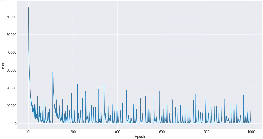
수행 결과 다음과 같은 loss 흐름을 보이며 학습이 진행 되었습니다.